This page provides a very brief historical background the project.
The modern field of mathematical evolutionary theory began to emerge just over 100 years ago, when W. Weinberg and G. H. Hardy independently showed how Mendelian genetics (which had been "rediscovered" only a few years earlier) can be used to calculate the frequencies of genotypes given the frequencies of alleles in a large population of randomly mating individuals with no selection. This result became the foundation of theoretical population genetics.
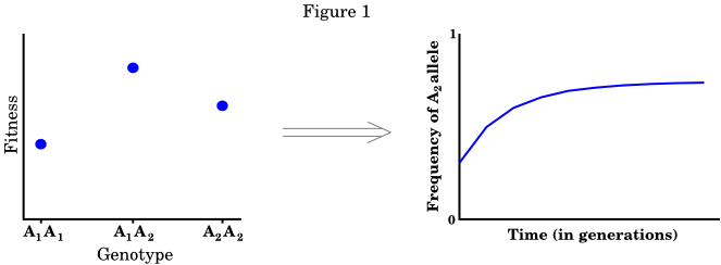
The reason that Hardy's and Weinberg's result is so important is that it allowed population geneticists to build mathematical theories of evolution that worked by tracking the frequencies, within a population, of alleles over time. Processes like selection, migration, and mating are usually thought of as taking place at the level of organisms, which to geneticists meant genotypes (the set of all alleles, at a particular genetic locus, in an individual - such as the pair of alleles that humans have at most loci, one coming from their mother and the other from their father). However, population geneticists found it much easier to follow the frequencies of alleles than those of genotypes (there are many more genotypes than there are alleles). The Hardy-Weinberg result allowed them to switch back and forth between genotypes (where most of the action is occurring) and alleles (which are easier to count). The basic approach of population genetics is illustrated in the following figure.
In the figure above, we start out by specifying the fitness values of each genotype in the population (for a single gene with two alleles, there are three of these). We then use the equations of population genetics to calculate the change in the frequency of one of the alleles from this. We then study evolution by following the allele frequencies over time.
In the subsequent decades, population geneticists extended the theory to include selection, drift, mutation, migration, nonrandom mating, multiple genes, and populations of finite size. In order to keep the mathematics tractable, these complicating factors are usually introduced one or a few at a time. Thus, models with nonrandom mating often assume infinite population size, models with drift and mutation often assume no selection, and so forth. The best way to include many factors in the same model has been to use the diffusion approximation, developed largely by S. Wright, M. Kimura, and S. Karlin. This is a powerful approach that allows us to study populations in which selection, drift, migration, and mutation are all happening. There is a catch, though, Diffusion theory works only if the total effect of all directional forces (selection, migration, mutation, etc.) is weak, and the population is large. In other words, we can combine many different processes only by assuming that their total effect is very small. Furthermore, nearly all of this theory was still based on the idea of following the frequencies of alleles (or sometimes haplotypes) over time, using the Hardy-Weinberg result to translate between allele frequencies and genotype frequencies. This approach became so ingrained that some textbooks even define evolution as change in allele frequencies.
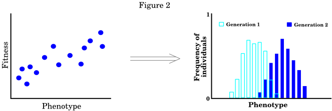
In 1970, George R. Price published a short paper that showed how a mathematical theory of evolution could be formulated in a completely different way. Price's equation considers only the phenotypes of individuals, the number of descendants that each individual leaves, and the phenotypes of those descendants. The resulting equation is usually written like this:
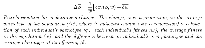
In Price's approach, every individual has a value for some phenotypic trait (such as body weight) and a fitness value (the number of descendants that it leaves). The idea is to take the distribution of phenotypic values and fitness values, along with the average degree to which offspring differ from their parents, and derive the change in the mean phenotype over a generation. By repeatedly applying the equation to different powers of the phenotype, the entire distribution of phenotypes in the next generation can be found. The following figure illustrates the approach.
Each dot in the figure on the left represents an individual in the population. The figure on the right shows the corresponding change, over a generation, in the distribution of phenotypes.
Beyond just showing that there is another way to do evolutionary mathematics, Price's equation has another distinguishing feature: it was derived without making any simplifying assumptions, including no assumptions about genetic transmission. It is thus an axiomatic theory in the sense that I am using that term. Because of this, the Price equation is actually much more general than it looks. For example, the "phenotype" can be any property of an individual that we can measure. It thus may be a morphological trait (such as body size), a behavioral trait (such as willingness to be altruistic), or a genetic trait (such as genotype). Similarly, "fitness is just the number of descendants that an individual has after some time interval. This may include offspring, grand-offspring, or even the individual itself at a later time.
The Price equation has been very useful because any evolving system, anywhere, must obey it. Price himself was primarily interested in the evolution of behavior, and many of the recent applications focus on things like the evolution of altruism. It is also possible to use this equation do derive the main results of quantitative genetics, and it is useful for studying cases in which selection acts simultaneously at different levels of organization.
Though the Price equation makes no simplifying assumptions, it does impose some limitations. Most notably, we need to know the exact value of each individual's fitness, and the exact degree to which their offspring differ from them phenotypically. This creates a problem, since before reproduction takes place, we can not know for sure how many offspring an individual will leave, or exactly what they will look like. Thus, Price's equation is exact only in hindsight; after reproduction has taken place (another way to say this is to say that the equation is deterministic).
It has long been recognized that evolution is a stochastic process, involving both predictable and unpredictable elements. The most well known stochastic evolutionary process is genetic drift, which plays a very important role in molecular evolution. The fact that the Price equation is deterministic thus limits its ability to serve as a unifying principle for all evolutionary processes. The starting point for a truly general axiomatic theory of evolution is thus to derive a result analogous to the price equation, but for which each individual has a distribution of possible fitness values and another distribution of possible offspring phenotypes. In order to do this, both fitness and offspring phenotype must be treated not as specific values, but as random variables.