One of the important features of the axiomatic theory is that things like fitness, population size, immigration rate, emigration rate, and offspring phenotype are all treated as "random variables". This page gives a brief explanation of what this means, and why it leads to some unexpected consequences.
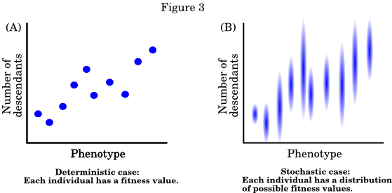
The simplest way to think of random variables is that they are terms to which we do not assign a numerical value (as we do to most variables), but rather a probability distribution of possible values. The following figure illustrates this for the case of fitness (here defined as number of descendants). Figure 3A shows the deterministic case, in which each individual has a specific fitness value. In Figure 3B, fitness is a random variable - each individual has a distribution of possible values (the degree of shading indicates probability).
Note that in Figure 3B, individuals may differ not only in their expected fitness values (the means of their fitness distributions), but also in the shape of their respective fitness distributions (measured by the variance and other moments). This is why evolutionary processes appear when we treat fitness as a random variable that are invisible when we treat it as a specific value.
Random variables need to be treated differently from variables that take a numerical value. This is especially important when we are calculating the expected value of the product or the ratio of two random variables. For example: if a and b are random variables (such as an individual's fitness and the phenotype of its offspring), then the expected value of a times b [written E(ab)] is not just the product of the expected values. Rather:
E(ab) = E(a)E(b) + cov(a, b)
Where cov(a, b) is the covariance between a and b. This makes sense when we recall that, since both a and b have associated distributions, their distributions could be correlated with one another.
Things get substantially less intuitive when we are dealing with the ratio of two random variables. Here, even if a and b are not correlated (so that cov(a, b) = 0), the expected value of the ratio is still not equal to the ratio of the expected values:
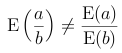
Failure to appreciate this fact has led to much confusion. In fact, there is a paradox in philosophy, called the "Two Envelope Paradox", that is a result of a failure to correctly calculate the ratio of the expected values of two random variables. (I discuss the two envelopes paradox, and show how to resolve it, at the end of this essay).
The reason that I bring all of this up is that one of the central terms in the axiomatic theory is the expected value of the ratio of two random variables ( , the expected value of individual fitness divided by mean population fitness). The equation for is rather complicated. For our purposes here, what matters is that it is a function of each individual's fitness distribution. The evolutionary consequences of this fact are discussed in the next section.
Directional stochastic effects
These are directional evolutionary processes (meaning that the expected change in mean phenotype is not zero) that result from differences in the shapes of fitness distributions between individuals. Many of these effects have emerged so far in this project - all but one of them previously undescribed.
Directional stochastic effects resemble drift in that they appear only if there is some stochastic variation in fitness. On the other hand, they resemble selection in that they can be directional (drift is generally defined as non-directional). Based on reviewers' comments for manuscripts and grants, some of my colleagues think that these should all be classified as kinds of selection, while others think that they are all just different kinds of drift.
The figure below illustrates a simple example in which individuals with different phenotypes have the same mean fitness, but differences in the variance in fitness drive directional change. In this case, there are two phenotypes in the population, 0 and 1, at equal frequency. Individuals with phenotypic value 0 have a 50% chance of leaving no descendants and a 50% chance of leaving two descendants. Their mean fitness is thus equal to 1. Individuals with phenotypic value 1 have a 100% chance of leaving one descendant, so their mean fitness is also equal to 1.
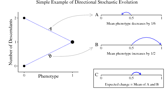
For the moment, let's consider the case in which all individuals with phenotypic value 0 have the same fitness at any given time (i.e. they all have w = 0 or they all have w = 2). There is a 50% chance that phenotypic value 1 will increase in frequency and a 50% chance that it will decrease. However, when it increases, the mean phenotype (which is initially 0.5) increases to 1, so the change is +1/2. By contrast, when phenotypic value 1 decreases in frequency (when individuals with phenotype 0 each leave two offspring), the change in mean phenotype is -1/6. Since the expected change is just the average of these two outcomes, we find that the expected change is +1/6, even though both types have the same mean fitness.
[Note: this is not a consequence of the fact that phenotype 0 can have zero fitness. Also, this is not a result of selection favoring the phenotypic value with the highest geometric mean fitness. This last fact is illustrated in Rice 2008]. The example given above shows a case in which there is an expected directional change resulting from the fact that different phenotypes have differently shaped fitness distributions, even when the mean fitnesses are the same. There are many more complicated examples of directional stochastic effects, but all can be understood as cases in which the magnitude of change (the "step size") is different when a particular trait increases in frequency than when it decreases in frequency.
This is a puzzle in which there appear to be convincing arguments for different, incompatible, conclusions. As in all such cases, there is a flaw in at least one of the arguments. Finding the flaw illustrates the counterintuitive properties of ratios of random variables.
The scenario is this: You are presented with two envelopes, labeled 'A' and 'B', and told only that:
1) Each envelope contains some money.
2) One of them contains twice as much money as does the other.
You are not told which has more money. You are now told that you may choose only one of the envelopes and keep the money inside. You choose envelope 'A', and find that it contains $10. You are about to take the money when it is pointed out to you that, according to the rules of the game, you are allowed to switch envelopes if you wish, but you can switch only once (so you can't check out B and then switch back to A if B had less money).
The question is: Should you keep your $10, or trade it for whatever is in envelope B?
Argument for switching
Some philosophers have argued that, since envelope A is known to contain $10, and we were told that one envelope contains twice as much money as the other, envelope B must contain either $5 (with probability 0.5) or $20 (also with probability 0.5). The expected value of the monetary content of envelope B is thus the average of 5 and 20, which is $12.50. Since this value is larger than the $10 that you now have, you should switch.
Argument for not switching
Most people's intuition is that there is no advantage to switching. You have no way of knowing which envelope contains the most money, so you had a 50% chance of picking the best one. Furthermore, though you know that the envelopes contain different amounts of money, the distribution of possible values is the same for each of them - each has a 50% chance of containing x dollars and a 50% chance of containing 2x dollars. The fact that you don't know what x is should be irrelevant. Since the distributions are the same, their expected values are the same, so there is no reason to switch. This symmetry is apparent when we imagine that you first chose B instead of A. Regardless of how much money you find in B (so long as it is an even number of cents), the same argument for switching would apply.
Resolution
The correct answer is that there is no benefit to switching. The expected amount of money in envelope B is the same as the amount in envelope A. But what about the argument for switching? There does not appear to be any error in our calculations. The problem is that the argument for switching calculates the wrong value. In determining which envelope to choose, what we want to know is the ratio of their expected values, or E(B)/E(A). What we actually calculated, though, is the expected value of the ratio, or E(B/A). As mentioned above (and demonstrated here), these are not the same thing. To check that this explains the discrepency: Consider the case in which A and B have the same distribution, 50% chance of having value x and 50% chance of having value 2x, but are perfectly negatively correlated with one another (A contains x whenever B contains 2x, and vice versa). In this case, E(B)/E(A) = 1, and we can use Equation 11 in the derivation sheet to calculate E(B/A). Doing so yields E(B/A) = 1.25, which explains our (mis)calculated value of the $12.50 for envelope B.