Example
An ongoing experiment has been selecting for increased oil content in corn.
The top graph shows the distribution of sizes in the parent generation (in 1899).
When the largest parents were collected and used to produce the next generation, the offspring distribution is shifted to the right, but not as far as the selected parents were (because h² < 1).
 
 

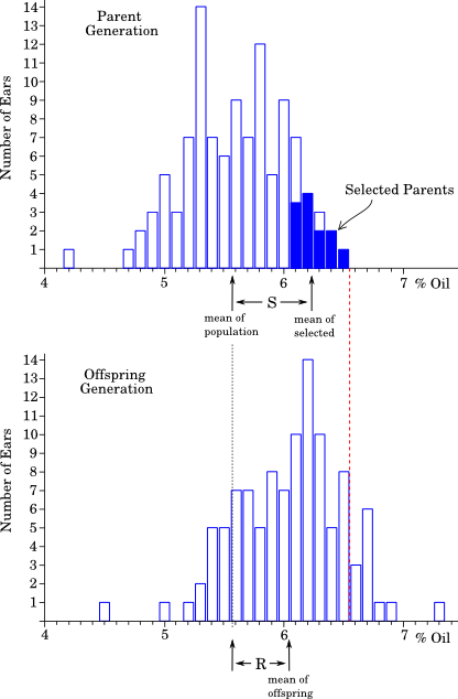
More importantly, note that in the parent generation there were no individuals with more than 6.5% oil. By contrast, in the offspring generation, there were an number of individuals with higher values than this (to the right of the dashed line).
Thus: New phenotypes appeared as a result of directional selection.

An important observation, from lab and agricultural studies, is that the variance in a population changes much more slowly than the mean .
This means that:

• New phenotypes are being produced each generation.
• The population can continue to evolve, without using up all of its genetic variation.

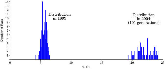
This experiment has been continuing for over 100 years (though they stopped durring World War II). Over time, the entire distribution moved such that there was no overlap with the original population. After 101 generations of selection, the mean had increased by about a factor of 4, and the distribution was far from where it started:

The new variation is produced by mutation (remember that many loci are involved) and, more importantly, by reshuffling of alleles.

Consider a population of size N = 10,000 with two loci, A and B, that contribute to size such that the A₂ and B₂ alleles both lead to larger individuals.
If A₂ and B₂ are both initially rare, then we expect to see some individuals that are heterozygous for one or the other, but no other combinations. If we select for larger size, then these alleles will increase in frequency, leading to the appearance of new genotypes.

Let p = freq(A₂) = freq(B₂)
(we are assuming that they are the same purely for convenience).

As p increases, new genotypes appear:
p < 0.005 : Some single heterozygotes. (A₁A₂ B₁B₁ and A₁A₁ B₁B₂)
p > 0.005 : Some double heterozygotes. (A₁A₂ B₁B₂)
p > 0.0072 : Some single homozygotes. (A₂A₂ B₁B₁ and A₁A₁ B₂B₂)
p > 0.029 : Some homozygote + heterozygotes. (A₂A₂ B₁B₂ and A₁A₂ B₂B₂)
p > 0.1 : Some double homozygotes. (A₂A₂ B₂B₂)

If there are many loci that each contribute a small amount to the trait, then recombination combined with slow increase in the frequency of alleles for large seeds will keep producing new variants for many generations . This provides enough time for mutation to produce new (initially rare) alleles, so the process continues.

Note that this production of new phenotypes is largely a result of the production of new combinations of alleles, which is only feasible with sexual reproduction .

The general case

We will designate phenotype with a Greek "phi",

Offspring phenotype will be denoted ^o

Sometimes, change in the environment, or directional mutation, can cause the entire population to change as a unit, we denote this change with a lowercase delta ()

With this notation, we can write the most general mathematical description of evolutionary change, known as the Price equation (Price, 1970)

The change in mean phenotype over a generation, which is the same as the "response to selection" (R), will be written as .

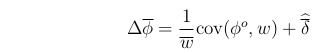
This equation makes no simplifying assumptions, and so applies exactly to any evolving system.

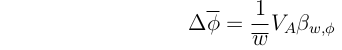
The standard assumptions of quantitative genetics are that offspring phenotype is a linear function of parent phenotype (with slope h²) and that = 0.
Imposing these assumptions on the Price equation yields:

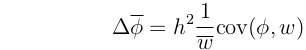
This is another way of writing the Breeder's equation.

Additive Genetic Variance

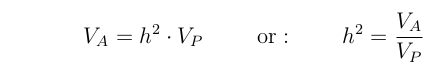
Define Vp as the total phenotypic variance among the parents. Then we define the "additive genetic variance" (V_A) as the portion of this that is predictably passed to the next generation.

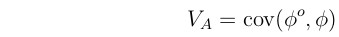
Alternately, we can think of the Additive genetic variance as being the covariance between parents and offspring.

Now, recall the version of the Breeder's equation that we derived from the Price equation:

With a bit of arithmetic, these last two equations can be rearranged to yield:

Note that this is a general case of:

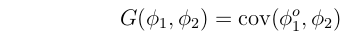
Multiple Characters:

Just as we can talk about the covariance of a trait in parents and their offspring ("Additive Genetic Variance") we can also consider the covariance of one trait, ₁, in the offspring with another, ₂, in their parents. This is often referred to as "Additive Genetic Covariance", denoted G(₁,₂):

Partial regression
Recall that the regression of x on a is the slope of the best fit line through the distribution of x and a.

If there are many variables (a, b, c, etc.) that x is related to, then we calculate the partial regression () of x on each variable.

Just as we found a best fit line relating x to a, we can find a best fit plane relating x to a and b simultaneously. The partial regressions are the slopes of this plane in the directions of the a axis and the b axis.

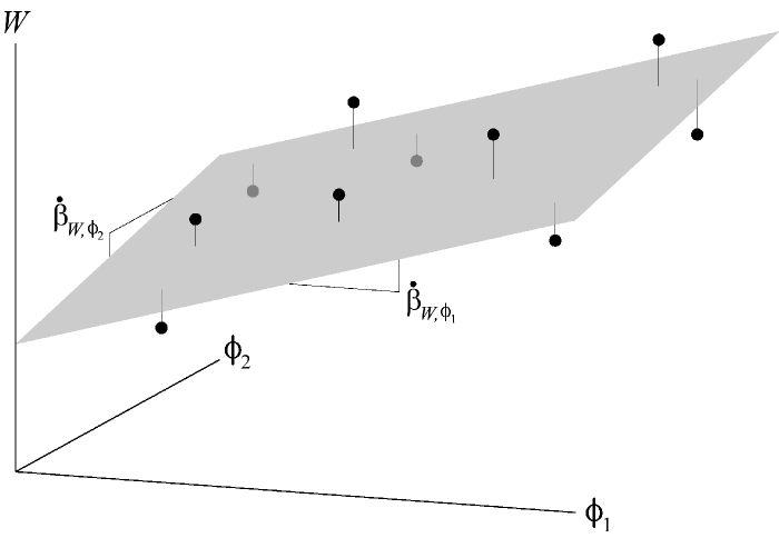
For x and two other variables, a and b, the partial regression of a on x is the slope of the best fit line relating a and x holding b constant.

Consider two characters, ₁ and ₂. Using additive genetic variances and covariances, We can write (recalling the one character equation):
 
 

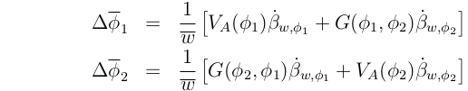
These equations account for the effects of both direct selection on a trait, and selection on another trait with which it genetically covaries.

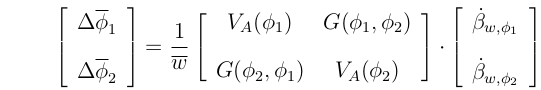
In matrix notation, this becomes:
 
 

Or, simply:

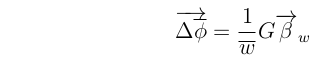
Here, the vector of partial regressions of fitness on the phenotypes:

is the Fitness Gradient; a vector pointing in the direction of maximum increase in fitness.