Recall Coalescent theory

An example of the coalescent is the "Mitochondrial Eve" - common ancestor of all mitochondria in the current human population who lived in Africa between 100,000 and 200,000 ya. This individual is also known as mtMRCA (mitochondrial Most Recent Common Ancestor).

Note that this individual was the common ancestor only for all modern mitochondria. Other parts of the genome can have different coalescent trees.

To see this, note that there must also be a tree for the Y chromosome, which must be different because the coalescent point must have been in a man, whereas the mitochondrial coalescent must have been in a woman.

Our discussion of coalescent theory assumed that population size is constant and that any gamete could combine with any other gamete (random mating). For such an idealized population, the probability that two gene copies coalesce in the previous generation is:

P_c = 1/(2N).

To make things a bit more realistic, we consider:

Effective Population Size (N_e)

For a real population that violates some of our assumptions, N_e is the size that an idealized population would have to be in order for it to behave the same (with respect to drift) as the real population.

Population size entered our calculations so far through it's influence on the probability that two lineages coalesce in a single generation. We thus seek a value of N_e that we can substitute for N in our previous calculations and have the results apply to more complex populations.

By definition:     P_c = 1/(2N_e)

Example 1:
Obligately outcrossing organisms with separate sexes.
N_f = number of breeding females
N_m = number of breeding males

so: 1/N_e = 1/(4N_f) + 1/(4N_m)
or:
 

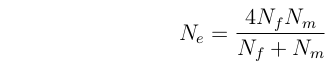
Note that if N_f = N_m = N/2, then  N_e = N
If N_f >> N_m, then N_e ~= 4

This can be a particular problem in the breeding of livestock, as well as in populations in which most males never breed.

Example 2:
Population size varies over time.

Consider a population that fluctuates in size over a period of t generations. (i.e. it has sizes N₁, N₂, ..., N_t).

Then if P[coalescence] is small in any one generation:

P[coalesce] = 1/(2N₁) + 1/(2N₂) + ... + 1/(2N_t) = t*[1/(2N_e)]

So:
 

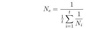
This is the Harmonic Mean of population size over time; strongly influenced by small values.
Example: Over 6 generations, N = 100, 100, 10, 10, 100, 100.
Arithmetic mean = 70
Harmonic mean = N_e = 25

------------------------------------------------------

Selection

Selection refers to differential survival or reproduction of individuals that is causally influenced by variation in some phenotypic trait.

Note that the causal influence of some phenotypic trait is essential; mere differential survival or reproduction could be random, producing drift.

If a trait has the property that it causes individuals that possess it to have a higher average survival or reproductive rate than individuals that lack it, then we say that there is selection for that trait.
Note that this is not necessary for a trait to increase in frequency. It may increase by drift or may be correlated with another trait that is selected for.

Selection may act at different stages of the lifecycle:

Viability selection - Differential survival (causally influenced by variation in phenotype) from zygote to reproductive age.
Sexual selection - Differential mating success (causally influenced by variation in phenotype), given that the individual has survived.
Fertility selection - Differential production of offspring (causally influenced by variation both parent's phenotypes), conditional on having survived and mated.

For the next few lectures, we will focus on selection acting at the level of individual diploid organisms.

We will consider only viability selection now. Sexual selection will be discussed later and we will not cover fertility selection in this course.

Closely related to the theory of selection is the concept of fitness.
Fitness measures an individual's expected contribution to the next generation.
Or: Expected lifetime reproductive success.

Modeling selection:

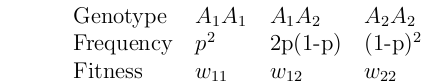
Consider a locus, A, with two alleles, A₁ and A₂.

Define p = frequency of A₁ alleles in the population.

Assign fitness to each possible genotype.
Fitness = expected number of offspring.

Other than introducing selection, we assume Hardy-Weinberg conditions:
Very large population
No migration
Random mating
Ignore mutation
Mendelian transmission

The frequencies are for zygotes, so with viability selection, we expect H-W frequencies so long as there is random mating (i.e. selection has not yet acted in this generation.)

Absolute fitness: Measures the average number of offspring for individuals with particular genotype.

Absolute fitness relates to population growth:

Relative fitness = absolute fitness scaled in some way that is convenient.
For example, we can divide all fitness values by the largest value, meaning that the most fit individual would have relative fitness of one.

In the theory that we will develop, we may use either absolute or relative fitness values without changing the results.

A term that will arise repeatedly is the Mean Population Fitness, denoted and defined as:

Let N be population size, then over one generation:

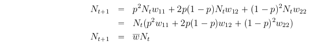
Thus, is the per capita population growth rate. Jul 8, 2021