Center for Emerging Energy Sciences

                     

Projects  -  Precision Metrology & Precision Measurement Science:

Calorimetry

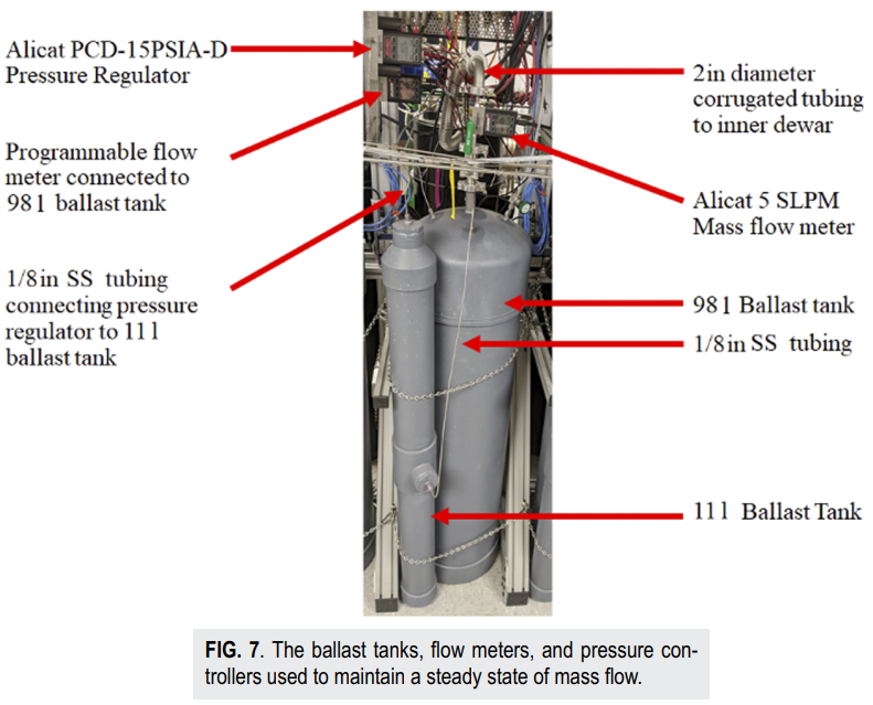
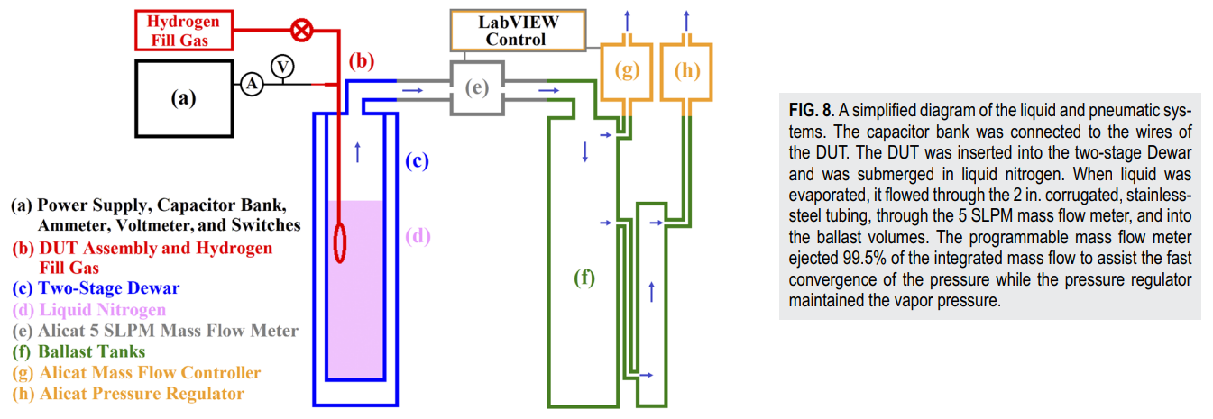
Fast-response nitrogen calorimeter and electric pulsing systems

      

 

Vacuum Calorimeter

An open-system differential vacuum calorimeter was design and developed at our laboratory. A calorimeter is used to measure the heat output of a system contained within the calorimetric boundary. The calorimeter is contained within the vacuum vessel, and operated in the Knudsen regime, to eliminate nonlinear convective losses. Superinsulation has been used to reduce radiative transfer with-in the vacuum vessel. A differential calorimeter approach was used to improve the calorimetric response via common-mode rejection. 

A scroll pump (Edwards nXDS15i) and 6-inch turbomolecular pump (Varian Turbo-V 300HT) are used to achieve high vacuum (1E-7 torr). Commercially available thermoelectric modules (TEM) are used both as passive heat-flux sensors as well as active heat pumps. The heat pumps are utilized to control an isothermal reservoir to provide a reference temperature for the passive TEMs. A custom fabricated liquid cooled heat-sink has been utilized to remove waste heat generated by the heat pumps. The active TEMs are controlled via a bipolar proportional-integral-derivative (PID) controller (TE Technology TC-720); the control reference is a 15 kΩ thermistor embedded into isothermal reservoir. 

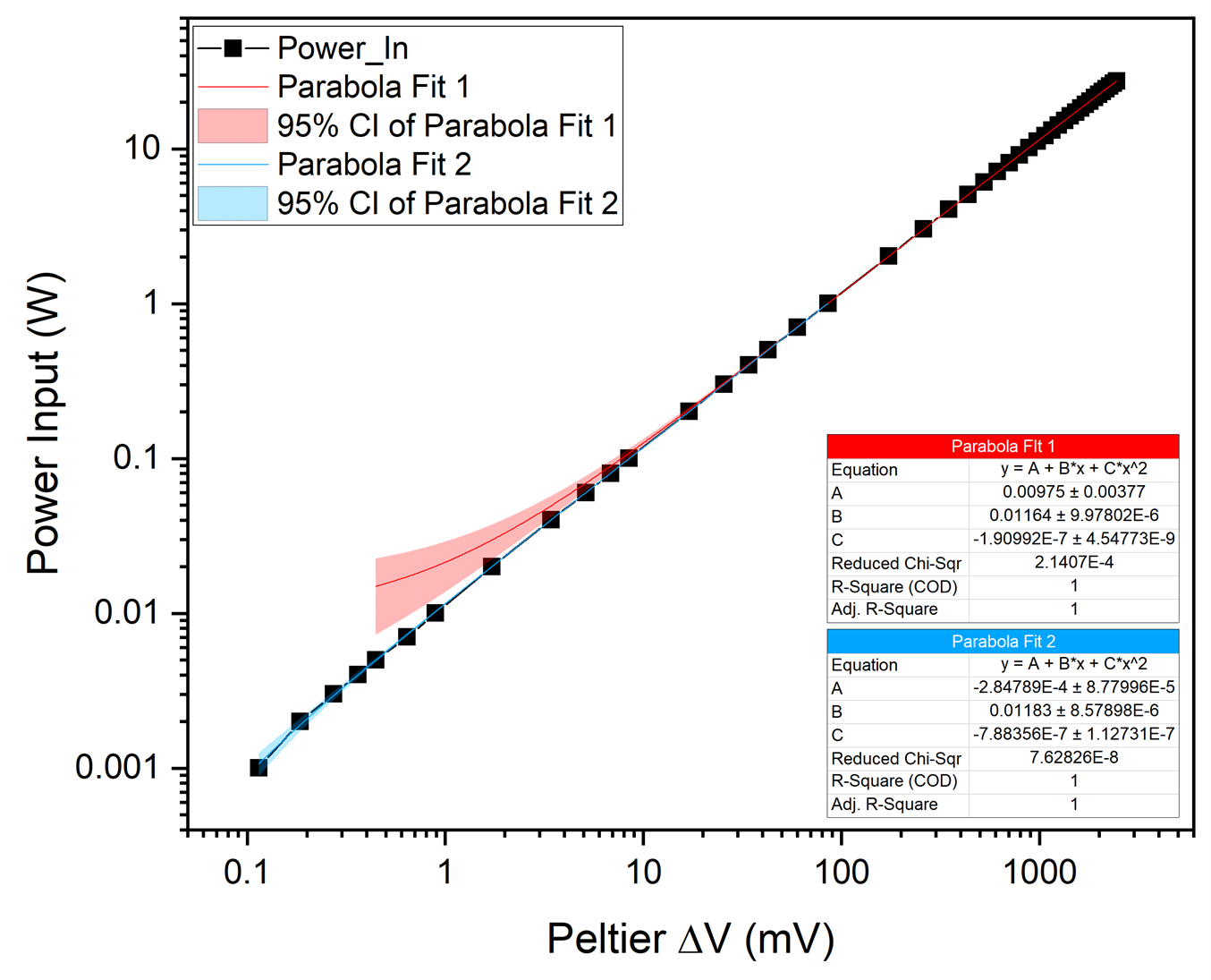
The calorimeter was designed to house two containers, an active container, and a control container. Two different container styles were also evaluated: a wet container used for electrochemical cells, and a dry container used for gaseous environments. Operating temperature is limited to 250 °C because of the heat pumping capability of the TEMs used to control the isothermal reservoir temperature. The calorimeter was designed for input powers ranging from 1 mW to 28 W; polynomial calibration up to 28 W yielded a Pearson's r exceeding 0.99999.

   

 

 

Electrochemical Calorimeter

 

Cold-Plate Open System Differential Calorimeter

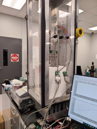
The CEES researchers and engineers have also designed, built, and tested a very accurate and sensitive open system calorimeter that operates in a normal room environment to measure the power and energy of a physical mass system. The calorimeter is unique in that it allows the measurement of energy and power from an ‘open' system, where mass and/or heat may enter and leave the calorimetric boundary (in a well-controlled manner). It is also novel in that it utilizes a solid-state heating and cooling thermoelectric assembly that acts as an electronically controlled heat reservoir. This calorimeter is capable of measuring power levels from a few milliwatts up to several watts, and it has been designed and optimized to be nearly immune to variations in ambient temperature and airflow. The calorimeter was modeled using lumped parameter electrical-thermal equivalent circuits in SPICE software. This modeling in the electrical domain led to the use of a mathematical correction factor that mitigates mismatches in thermal conduction paths between the active and the passive cell, as well as correcting for differences in the sensitivities of the flux sensors employed for heat flow measurement.

A simplified diagram of the open system differential calorimeter is shown below (figure 5). The calorimeter has two containers of arbitrary shape (cylindrical in this case for the type of experiments performed initially by CEES), that are in good thermal contact with the top of their respective heat flux sensors (not visible in image), while the other side of the sensors are connected to an active, electronically controlled Thermo-Electric Cold-Plate (CP). An experiment where heat or power output is to be measured is placed in the active, or working container, while the passive, or reference container is filled with a substance/material that approximately mimics the heat capacity and thermal resistance of the active experiment. In concept, common environmental or instrumental fluctuations register on both the experimental and reference containers, so, with proper sensitivity balance, these spurious fluctuations may be cancelled by rejecting the common mode. Not shown in the figure is the thermal insulation that is placed around each respective container to eliminate ambient convective interference.

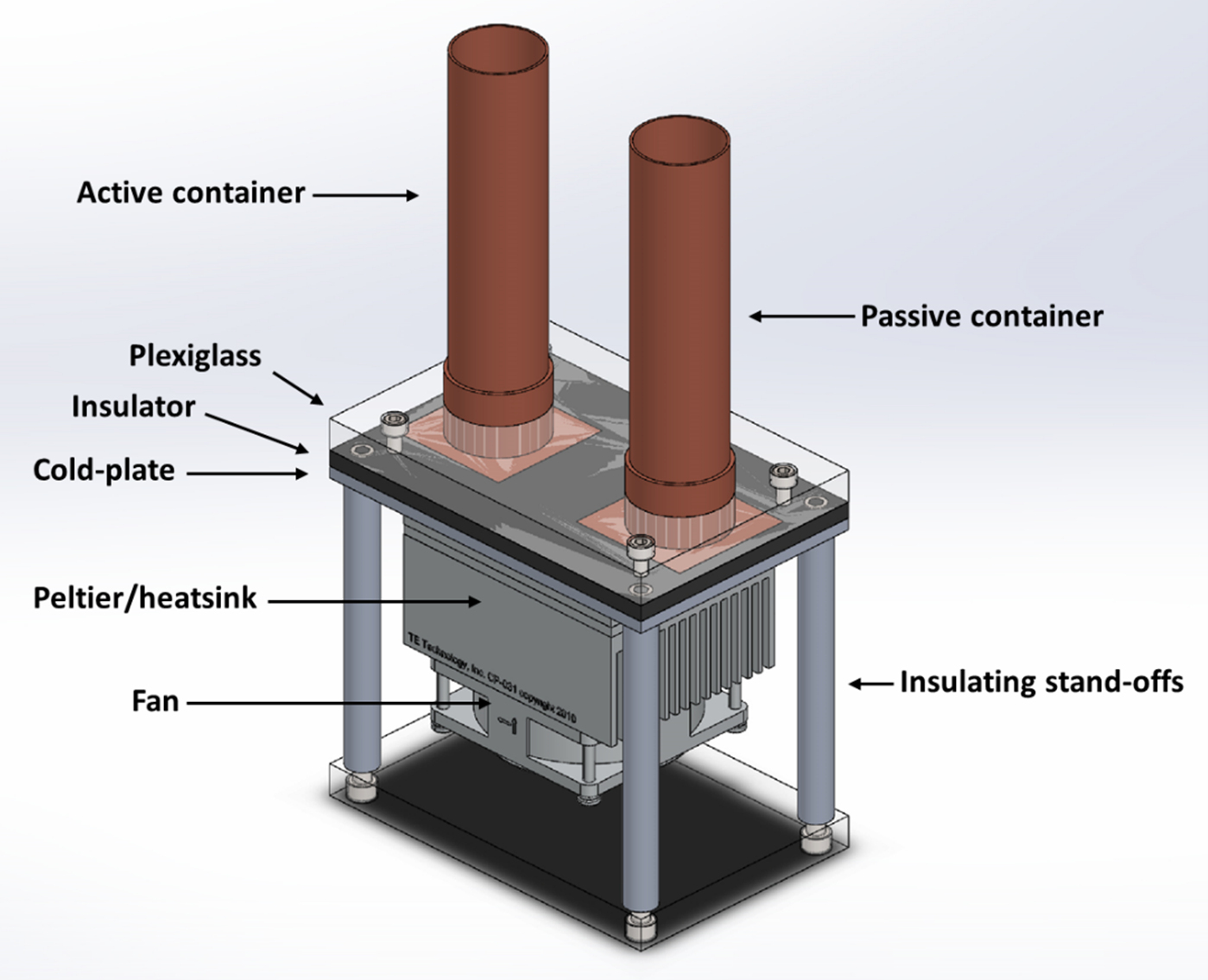
3-D Rendering of the Open System Differential Calorimeter

Each heat flux sensor develops a voltage output that is linearly proportional to the difference in temperature across its plates (ΔT). The difference between the active and passive heat flux sensors is obtained and scaled to produce a signal that is proportional to the power evolved in the active container. The use of a passive container of roughly the same thermal characteristics as the active allows the subtraction of ambient temperature perturbations; in effect giving the system Common-Mode Rejection (CMR) to heat flow.

The design of the calorimeter is highly innovative, and many of the innovations arose from performing various simulations of the heat flow using a lumped-parameter electrothermal equivalent model. Its use in the development of the calorimeter was not to determine absolute values for heat flow, temperatures, etc., rather it was used to ascertain the behavior of the system and the overall result of variations in ambient temperature and of mismatches in the thermal properties of the active and passive containers on the calculated output power. In this regard, the electrical equivalent modeling turned out to be a highly useful tool by producing a mathematical method for improving CMR.

Lumped parameter electrical equivalent thermal element modeling is based on the similar mathematical relationships that exists between one dimensional conductive heat flow driven by a temperature gradient to one dimensional electric current flow driven by an electric potential gradient. The thermal relationship is expressed compactly by Fourier's law of heat conduction:

Q_cond = -kA dT/dx

Where k is the thermal conductivity and A is the area normal to the direction of the heat flow. For the conditions cited above, the heat flow is a constant, making the temperature gradient also constant. This leads to a simple relationship between the heat flow through a piece of material, the temperature difference developed across it, and the physical dimensions of the material that correlates nicely to the interrelationship between current, voltage and resistance, respectively, as illustrated below.

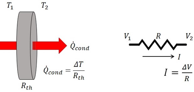
Thermal – Electrical Analogy

The thermal resistance, much like electrical resistance, depends on the material (thermal conductivity) and the physical geometry through which heat conduction takes place. A similar electrical-thermal equivalent relationship exists for both convection and radiation of heat from the surface of a material, for which only the surface area of the material affects the equivalent lumped thermal resistance of a given shape. For the simulations performed in this paper, only convective heat transfer was included in the model along with heat conduction. Convection is also a relatively strong function of temperature, and this effect is also included (as a linear function) in the SPICE model simulations.

There are likewise analogies for transient heat flow modeling using the concept of thermal capacitance as a lumped-parameter, but this is only modeled roughly in the simulations performed for the calorimeter and the time constant is scaled temporally to match the much faster paced simulations to the acquired data from actual experiments. If heat accumulated (Q) is of interest instead of the time rate of heat flow, there are quantitative ways of assessing the viability of using the thermal capacitance model to carry out transient analysis. This would be useful in the transient analysis if the heat capacity of the two containers is mismatched. Our interest is primarily in the steady-state results, but time dependent, transient effects may be modeled in the lumped-element of SPICE as thermal capacitances.

To perform the thermal equivalent simulations for the calorimeter, both the experimental system (contained in the active tube) and the calorimeter itself are broken into segments that are approximately delineated by isotherms where heat flow can be considered one–dimensional. Again, the simulations were intended to observe system response to altered parameters and external perturbations; better absolute accuracy could be obtained by increasing the number of elements corresponding to each physical segment. All simulations were performed in LTSpice software. The figure below displays a diagram of the cold-plate differential calorimeter with the electrical simulation schematic overlaid to show the correspondence between the electrical components and their approximate corresponding physical segments.

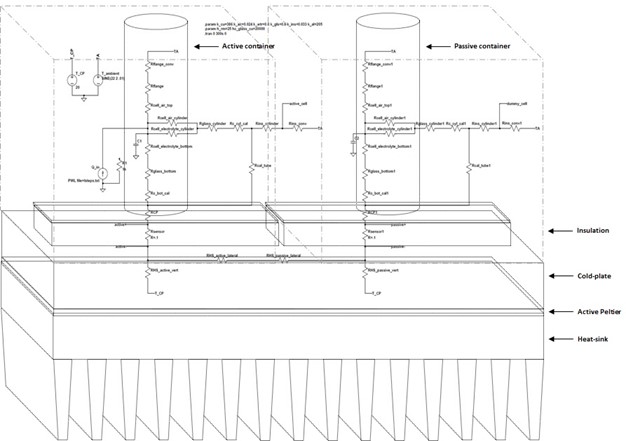
Physical Diagram with Electrical SPICE Model Overlaid

The ambient temperature, and the cold-plate set point, are modeled as ideal voltage sources, and input power is modeled as an ideal current source. Heat flux sensors are simply modeled as resistors, chosen so that the thermal resistance (°C/W) matches that of the physical flux sensor closely. The output of the heat flux sensors in the simulation is a temperature gradient (represented by a voltage in simulations) that is measured through the actual flux sensors linear output in voltage per Watt heat flow (V/W). The sources can easily represent their physical counterparts; ambient can vary arbitrarily, mimicking room temperature swings, and the cold-plate source can be varied in a fast manner to imitate fluctuations in the PID control system that regulates the cold-plate.

An example simulation is illustrated in the figure below, alongside actual data from a physical unit. The simulation shows a small (50mW) step in input power, and the corresponding waveforms from the flux sensors. 

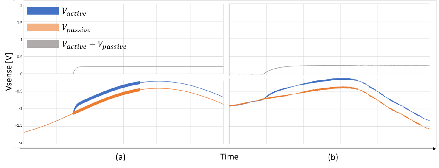
Simulation (a) versus physical (b) Data.

The slow, large swing seen in the output of the active and passive flux sensor signals is a variation in room temperature (TA source in the simulation), the low-level, fast perturbations are from the control system of the cold-plate (CP source in the simulation). When the active and passive heat paths are closely matched (see next section), both of these unwanted signals are rejected in the difference signal, ΔV_Sense.

While the use of an active cold-plate as a heat reservoir and a stable reference improved the accuracy of the calorimeter both in simulations and empirically, another source of error in such an open system, as mentioned in the preceding section, results from any asymmetry in the heat conduction and convection paths between the active and the passive containers to ambient temperature. This is easier to visualize if the entire simulation model for the calorimeter is dramatically simplified into an equivalent circuit that resembles an electrical Wheatstone-bridge circuit, as displayed in figure 9. This simplified analog model shows schematically how mismatched thermal resistance paths introduce errors; they cause a reduction in the differential circuits CMR by altering the systems' symmetry.

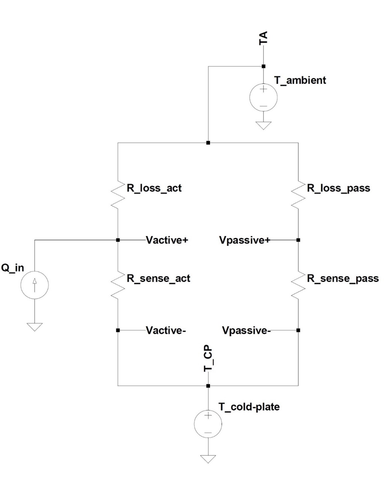
Simplified Equivalent Circuit

In order to reject the common mode signal (ambient temperature in this case) the ratios of each branch's voltage divider (thermal paths in the physical system) must be equal.  While it would be a physical impossibility to “trim” the thermal conduction and convection resistances, and perfectly match each flux sensor's sensitivity, a mathematical correction can be applied to the signal to regain good CMR in post-processing of the data. A simple reading of each sensor is taken with no applied input power (Q_in set to zero in simulations) and the ratio of average V_active to average V_passive is obtained. This correction factor is used to mathematically bring the circuit back into ‘balance.'  The following figure displays a simulation with the same temperature perturbation applied as in the previous simulations, but where an intentional (large) asymmetry was introduced by increasing the passive container's convecting surface area to ten times that of the active side, in effect decreasing R_loss_pass in the previous figure. Power input steps are grey, measured power out calculated without λ is the blue graph, and corrected power is the red graph.

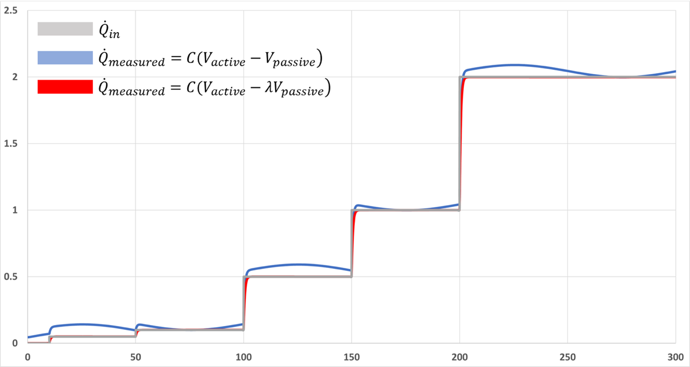
Intentional Asymmetry and Corrected Signal

As can be seen from the graph, the asymmetry caused by a larger convecting surface in the passive container leads to the ambient temperature perturbations coupling into the measured output signal. The correction factor mathematically restores the ratios of the thermal conductance paths and restores the calorimeter's CMR with the use of a simple initial measurement, and a slightly altered calculation of Q_measured.  More information on this particular instrument can be found in Review of Scientific Instruments, Vol 91, issue 9.

The electrical – thermal equivalent modeling used in the design of the differential calorimeter has been used in several other systems at CEES with equally useful results. This method offers nearly instantaneous simulation results, especially when compared to other methods such as COMSOL. It allows researchers to ‘see' subtleties in complex heat-flow systems, and understand interrelationships between variables intuitively.

---

 

 

 

---

Mass Spectrometry

Picomole-resolution mass spectrometers for light isotopes

CEES has both advanced mass spectrometer instruments and the necessary personnel with significant operational expertise.  Mass spectrometry, one of the generally applicable of all the analytical tools, has provided qualitative and quantitative information about the molecular and atomic composition of materials.  The main advantages of mass spectrometry as analytical technique have been its better sensitivity than other analytical techniques and its specificity in identifying unknows and in confirming the presence of suspected compounds.  The excellent specificity results from characteristic fragmentation patterns, which has given information about molecular and atomic weight and molecular structure.  As an added advantage, a mass spectrometer has become an essential instrument when used with stable isotopes in investigations of reaction mechanisms and in tracer detection.

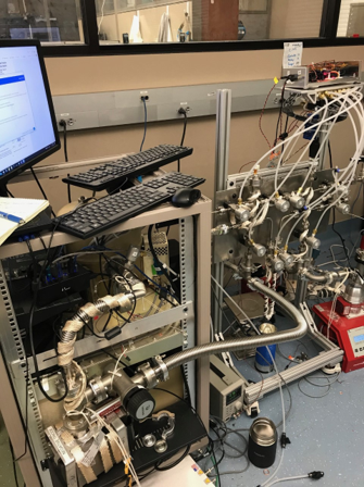
CEES has two distinct types of mass spectrometer instruments available for use in the composition determinations of gas mixtures.  Each instrument has its own dedicated sampling system with a vacuum pumping station.  Accurate, full-range gauges have measured the manifold pressures.  Likewise, a proportional temperature controller and heater provide thermal stability for each instrument and its manifold.

Residual Gas Analyzer

The first mass spectrometer is a quadrapole mass analyzer, also known as a residual gas analyzer (RGA).  It is a Stanford Research Systems model RGA300 with a faraday cup detector and an electron-impact (EI) ionization source used to generate the positive ions.  A calibrated leak valve interfaces it to a small sampling manifold with a turbomolecular pump used for evacuation.  A PC with software has provided instrument control and data acquisition.

The faraday cup detector is a simple and effective means for ion current monitoring.  The best characteristics of this detector include stability, simplicity, wide dynamic range, and lack of mass discrimination.  Regardless of their mass, all ions are detected with the same efficiency.

The commonly used electron-impact (EI) ionization source is an advanced ionization method.  Once past the calibrated leak valve, the neutral molecules enter a vacuum chamber and are exposed to electrons emitted from a glowing filament.  Ion formation occurs from the exchange of the energy during the collision of the electron beam and sample molecule.  The filament potential is variable, but 70 volts is commonly used.  This potential gives an appearance spectrum independent of the electric fields and this feature is necessary for the reproducibility required for quantitative work.

The model RGA300 has a mass range of 1 to 300 amu.  It has a resolution of 0.5 amu or better at 10% peak height.

Fourier-Transform Ion Cyclotron Resonance (FT-ICR) Mass Spectrometer

CEES has modified seven high resolution FT-ICR mass spectrometers for quantification of low mass species.  The original instruments, named advanced Quantra, were last manufactured by Siemens Industry, Inc. (Process Analytics) in 2008.  With an appropriate sampling system, they are capable of quantitatively measuring sub-picomole amounts of ⁴He and ³He in a hydrogen gas background.  The first of these instruments began operation in 2017, with six of them functioning through 2020.  Currently, four of these instruments are fully operational and have a custom inlet manifold containing a hydrogen removal getter for sample pretreatment.  In 2020, all four of these instruments were upgraded with additional cabling to improve the signal-to-noise ratio.  The resulting system exhibits adequate resolution and quantitative measurement capabilities to contribute significantly as a diagnostic tool within climate and energy research.  These high-resolution FT-ICR mass spectrometers have routinely achieved a resolution, R = m/∆m better than 10,000 at mass-3, with a mass resolution that scales as 1/m.  These devices have easily resolved D₂ from ⁴He, and DH from ³He.

   

            

 

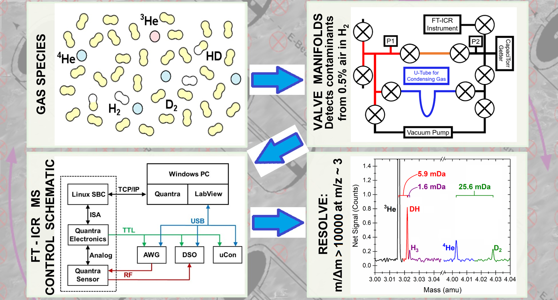
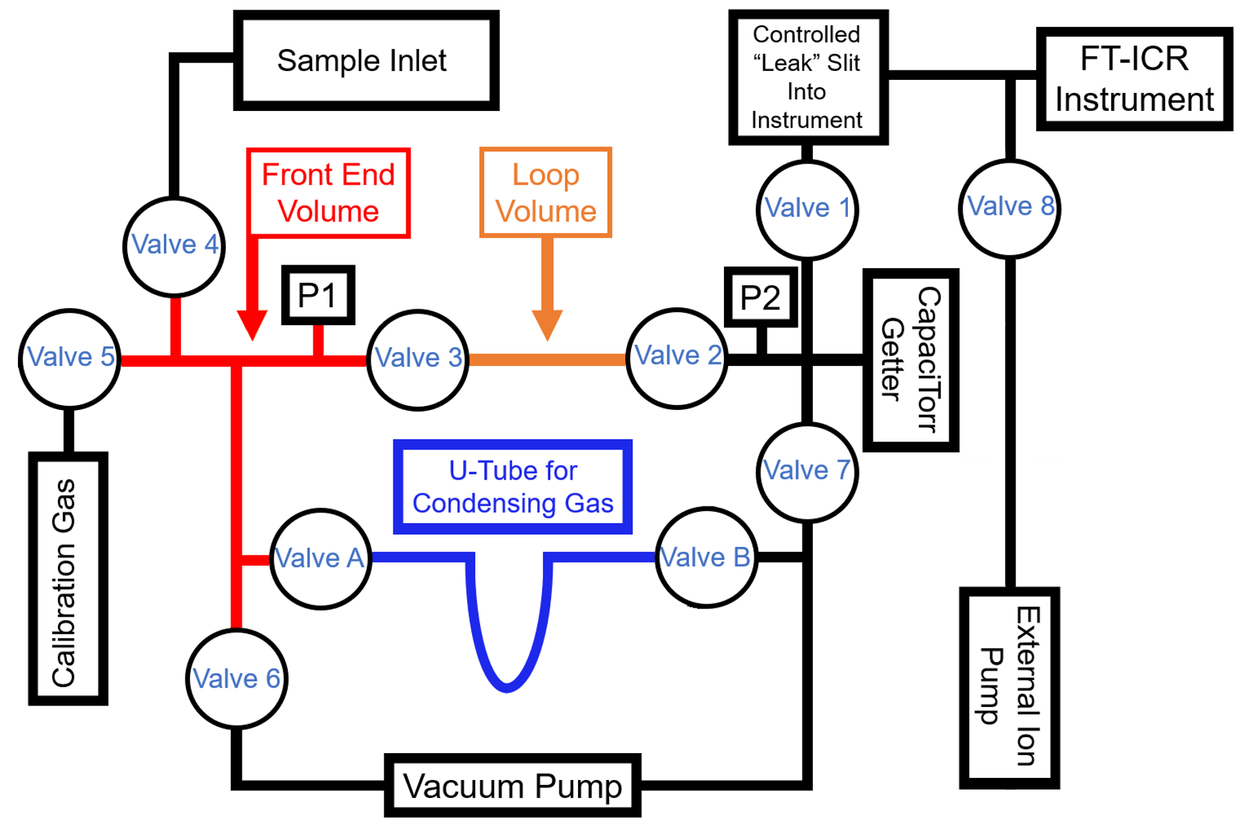
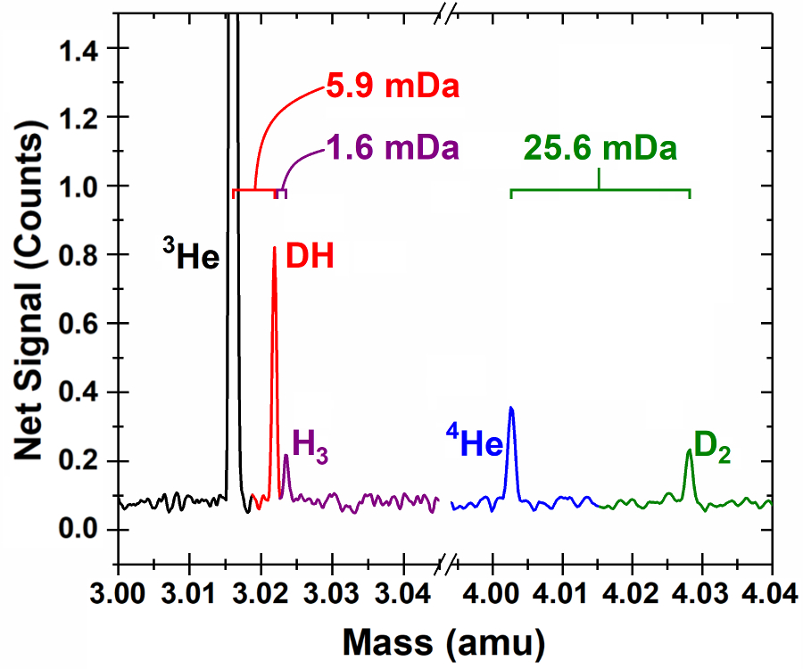
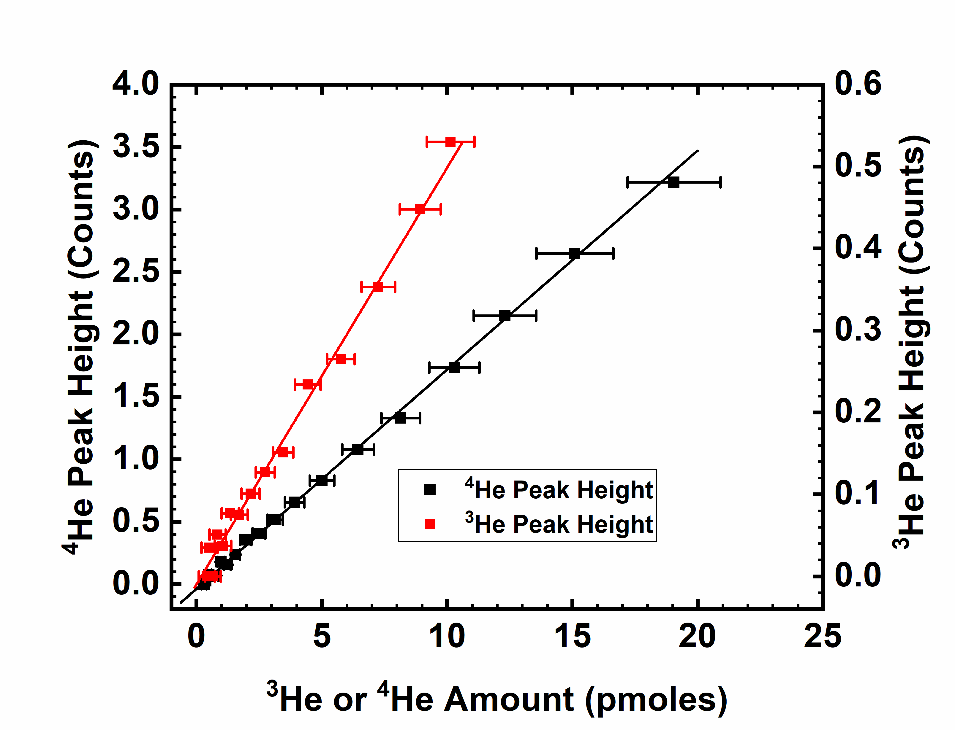
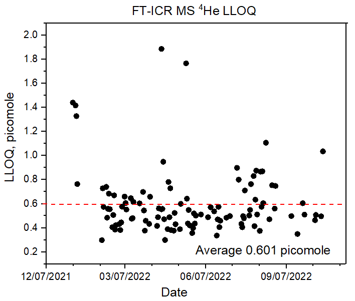
This system has also been used to measure ⁴⁰Ar and ²⁰Ne quantitatively, and these measurements have provided real-time air invasion detection into the sample and/or measurement system while helium measurements were being made.  While no concentration measurements of radioactive species have been attempted to date with this system, it is expected to easily resolve DT from D₂H (a 0.0059 Da mass difference) and HT from all other mass-4 species.  The linearity and stability of this system has been demonstrated through repeated periodic calibrations against a known dilute helium-in-balance-hydrogen external standard.  The lowest level of quantification (LLOQ) values for 4He is plotted below.  The average helium LLOQ value is 0.601 ±0.268 picomole.

 

 

 

 

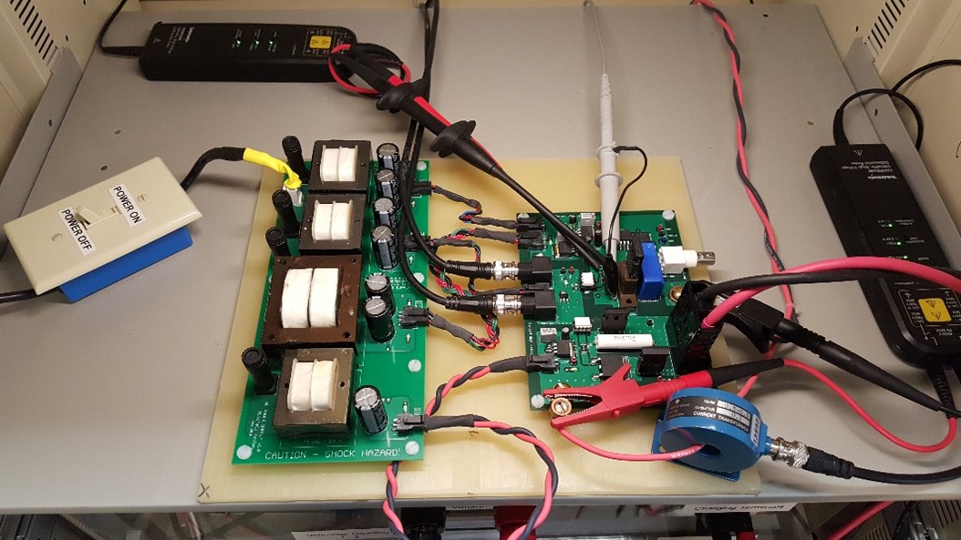
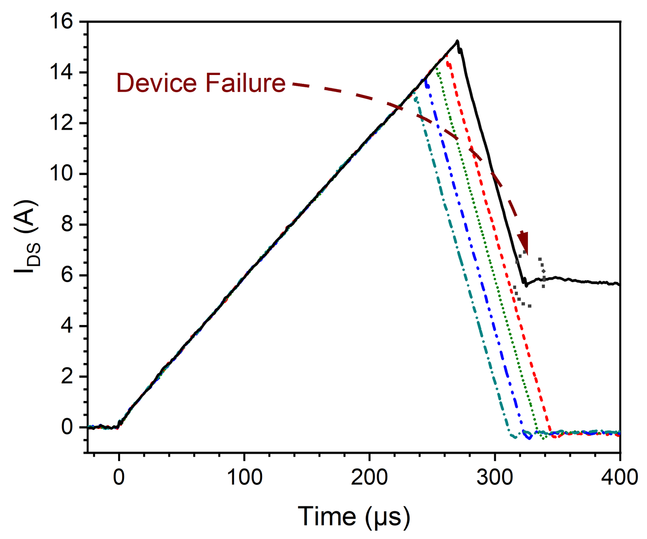
Wide Bandgap Avalanche Energy Test Bed

Custom electronic testbed utilized for the evaluation of avalanche energy tolerance of wide bandgap semiconductors. A modular design approach was utilized to allow for a wide variety of control conditions to be implemented in addition to varying package topologies. An important design aspect implemented was precise energy control allowing the failure mode to be analyzed post destructive failure. Both commercial and research grade Silicon Carbide (SiC) MOSFETs were evaluated.

Relevant Publication Links:

https://ieeexplore.ieee.org/abstract/document/7676377

https://www.sciencedirect.com/science/article/pii/S0026271417305693

 

 

 

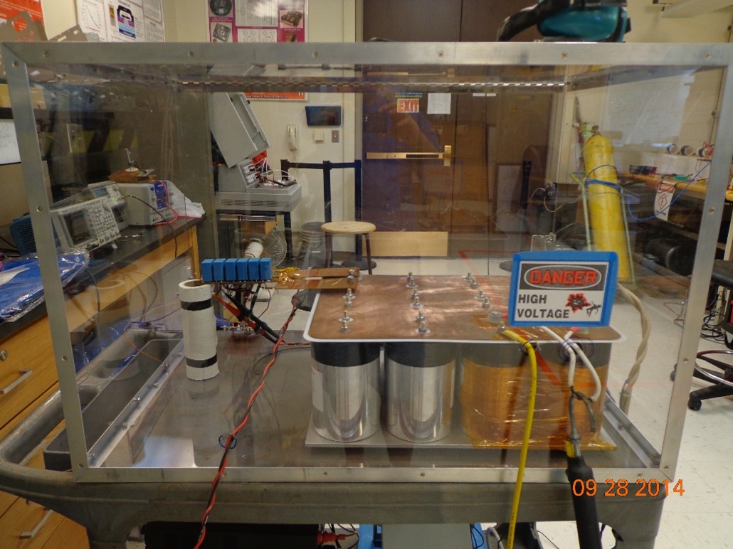
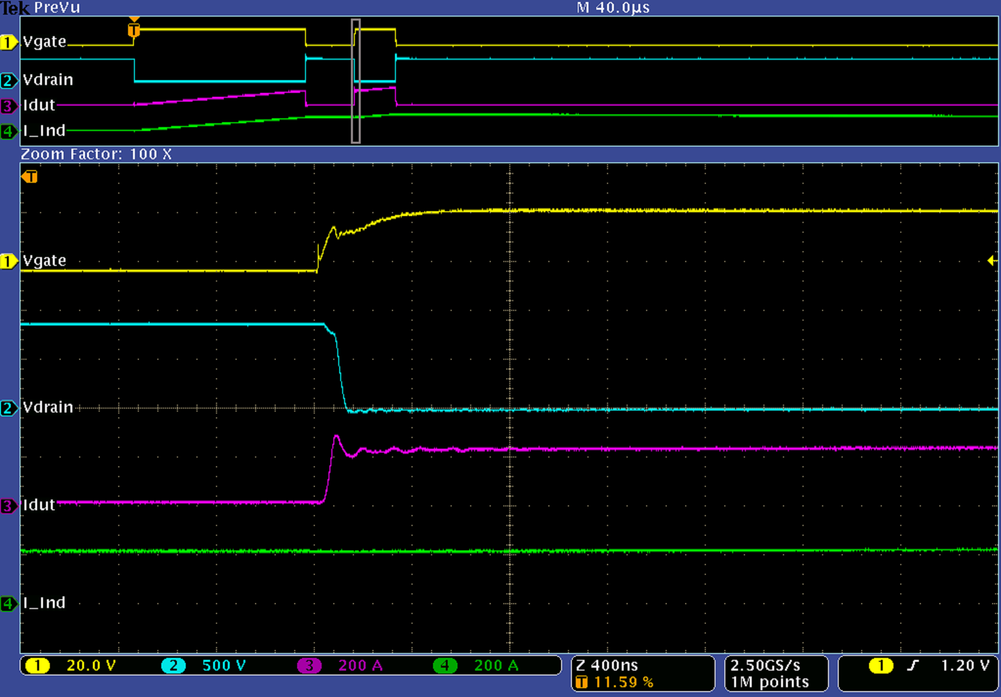
Low Inductance Double Pulse Test Bed

A low inductance double pulse tester was developed to analyze the switching characteristics of SiC MOSFET modules. The parallel configuration of the modules enables high current operation, however, a compatible power supply unit is often difficult to acquire. With a desired operating current of 300 A peak, a cost effective solution was to implement a capacitor bank as an energy source. A low inductance design was selected to minimize the effect of parastic inductance on measurement integrity. The system was designed to provide pulse widths up to 400 µs with a maximum current droop of only 2 %;  maximum design energy was ≈ 7 kJ.